使用 ecl EKF

官网英文原文地址： http://dev.px4.io/tuning_the_ecl_ekf.html

本教程旨在解答一些关于ECL EKF算法使用的常见问题。

什么是 ecl EKF?

ECL(Estimation and Control Library，估计与控制库）使用EKF(Extended Kalman Filter，扩展卡尔曼滤波器)算法来处理传感器测量信息并为下面的状态提供估计：

四元数，定义为从地球NED(北东地)坐标系到机体坐标系X,Y,Z的旋转四元数
速度，关于IMU - 北，东，地 (m/s)
位置，关于IMU - 北，东，地 (m)
角速度偏移估计，关于IMU - X,Y,Z (rad)
速度偏移估计，关于IMU - X,Y,Z (m/s)
地磁分量 - 北，东，地 (gauss)
磁偏量，关于飞行器本身 - X,Y,Z (gauss)
风速 - 北，东 (m/s)

EKF在一个延迟的fusion time horizon上运行，以允许传感器在每次测量时相对于IMU存在不同的时间延迟。每个传感器的数据都是FIFO缓存的并由EKF从缓存中检索，得以在正确的时候使用。每个传感器的延迟补偿由参数EKF2_*_DELAY控制。

互补滤波器用于利用缓存好的IMU数据将状态从fusion time horizon向前传播到当前时间。该滤波器的时间常数由参数EKF2_TAU_VEL和EKF2_TAU_POS控制。

注意：fusion time horizon延迟和缓冲区的长度由参数EKF2_*_DELAY的最大值确定。如果未使用某传感器，建议将其时间延迟设置为零。降低fusion time horizon延迟会减少互补滤波器中用于将状态向前传播到当前时间的误差

调整位置和速度状态以消除IMU和机体坐标系之间由于安装误差所产生的偏移，避免其输出到控制回路。 IMU相对于机体坐标系的位置由参数EKF2_IMU_POS_X，Y，Z设置。

EKF仅使用IMU的数据进行状态预测。IMU的数据不会用作EKF推导过程中的量测值。协方差预测、状态更新以及协方差更新的代数方程都是使用Matlab符号工具箱导出的，可以在这里找到：Matlab Symbolic Derivation

ecl EKF使用何种传感器测量值？

根据传感器测量值的不同组合，EKF具有不同的操作模式。在启动时，滤波器会检查传感器的最小可行组合，并在初始倾斜、偏航以及高度对准完成后进入一个提供旋转、垂直速度、垂直位置、IMU角增量误差和IMU速度增量误差估计的模式。

此模式需要有传感器的数据，例如偏航数据源（由磁力计或者外部视觉设备提供）和高度数据源。所有的EKF操作模式都需要这个最小的数据集。然后可以使用其他传感器数据来估计附加的状态。

惯性测量单元（IMU）

惯性测量单元的三轴位置固定，用于采集单位角增量和速度增量数据，最低采样频率为100Hz。

注意：在EKF使用IMU角增量数据之前应对其进行校正修正。

磁力计

三轴磁力计（或者是外部视觉系统）的最低采样率为5Hz。磁力计数据可以以两种方式使用：

Magnetometer measurements are converted to a yaw angle using the tilt estimate and magnetic declination. This yaw angle is then used as an observation by the EKF. This method is less accurate and does not allow for learning of body frame field offsets, however it is more robust to magnetic anomalies and large start-up gyro biases. It is the default method used during start-up and on ground.
使用倾斜估计和磁偏角将磁力计测量值转换为偏航角
The XYZ magnetometer readings are used as separate observations. This method is more accurate and allows body frame offsets to be learned, but assumes the earth magnetic field environment only changes slowly and performs less well when there are significant external magnetic anomalies. It is the default method when the vehicle is airborne and has climbed past 1.5 m altitude.

The logic used to select the mode is set by the EKF2_MAG_TYPE parameter.

Height

A source of height data - either GPS, barometric pressure, range finder or external vision at a minimum rate of 5Hz is required. Note: The primary source of height data is controlled by the EKF2_HGT_MODE parameter.

If these measurements are not present, the EKF will not start. When these measurements have been detected, the EKF will initialise the states and complete the tilt and yaw alignment. When tilt and yaw alignment is complete, the EKF can then transition to other modes of operation enabling use of additional sensor data:

GPS

GPS measurements will be used for position and velocity if the following conditions are met:

GPS use is enabled via setting of the EKF2_AID_MASK parameter.
GPS quality checks have passed. These checks are controlled by the EKF2_GPS_CHECK and EKF2_REQ<> parameters.
GPS height can be used directly by the EKF via setting of the EKF2_HGT_MODE parameter.

Range Finder

Range finder distance to ground is used a by a single state filter to estimate the vertical position of the terrain relative to the height datum.

If operating over a flat surface that can be used as a zero height datum, the range finder data can also be used directly by the EKF to estimate height by setting the EKF2_HGT_MODE parameter to 2.

Airspeed

Equivalent Airspeed (EAS) data can be used to estimate wind velocity and reduce drift when GPS is lost by setting EKF2_ARSP_THR to a positive value. Airspeed data will be used when it exceeds the threshold set by a positive value for EKF2_ARSP_THR and the vehicle type is not rotary wing.

Synthetic Sideslip

Fixed wing platforms can take advantage of an assumed sidelsip observation of zero to improve wind speed estimation and also enable wind speed estimation without an airspeed sensor. This is enabled by setting the EKF2_FUSE_BETA parameter to 1.

Optical Flow

Optical flow data will be used if the following conditions are met:

Valid range finder data is available.
Bit position 1 in the EKF2_AID_MASK parameter is true.
The quality metric returned by the flow sensor is greater than the minimum requirement set by the EKF2_OF_QMIN parameter

External Vision System

Position and Pose Measurements from an exernal vision system, eg Vicon, can be used:

External vision system horizontal position data will be used if bit position 3 in the EKF2_AID_MASK parameter is true.
External vision system vertical position data will be used if the EKF2_HGT_MODE parameter is set to 3.

* External vision system pose data will be used for yaw estimation if bit position 4 in the EKF2_AID_MASK parameter is true.

How do I use the 'ecl' library EKF?

Set the SYS_MC_EST_GROUP parameter to 2 to use the ecl EKF.

What are the advantages and disadvantages of the ecl EKF over other estimators?

Like all estimators, much of the performance comes from the tuning to match sensor characteristics. Tuning is a compromise between accuracy and robustness and although we have attempted to provide a tune that meets the needs of most users, there will be applications where tuning changes are required.

For this reason, no claims for accuracy relative to the legacy combination of attitude_estimator_q + local_position_estimator have been made and the best choice of estimator will depend on the application and tuning.

Disadvantages

* The ecl EKF is a complex algorithm that requires a good understanding of extended Kalman filter theory and its application to navigation problems to tune successfully. It is therefore more difficult for users that are not achieving good results to know what to change.

The ecl EKF uses more RAM and flash space
The ecl EKF uses more logging space.
The ecl EKF has had less flight time

Advantages

The ecl EKF is able to fuse data from sensors with different time delays and data rates in a mathematically consistent way which improves accuracy during dynamic manoeuvres once time delay parameters are set correctly.
The ecl EKF is capable of fusing a large range of different sensor types.
The ecl EKF detects and reports statistically significant inconsistencies in sensor data, assisting with diagnosis of sensor errors.
For fixed wing operation, the ecl EKF estimates wind speed with or without an airspeed sensor and is able to use the estimated wind in combination with airspeed measurements and sideslip assumptions to extend the dead-reckoning time avalable if GPS is lost in flight.
The ecl EKF estimates 3-axis accelerometer bias which improves accuracy for tailsitters and other vehicles that experience large attitude changes between flight phases.
The federated architecture (combined attitude and position/velocity estimation) means that attitude estimation benefits from all sensor measurements. This should provide the potential for improved attitude estimation if tuned correctly.

How do I check the EKF performance?

EKF outputs, states and status data are published to a number of uORB topics which are logged to the SD card during flight. The following guide assumes that data has been logged using the .ulog file format. To use the .ulog format, set the SYS_LOGGER parameter to 1.

The .ulog format data can be parsed in python by using the PX4 pyulog library.

Most of the EKF data is found in the ekf2_innovationsand estimator_status uORB messages that are logged to the .ulog file.

Output Data

Attitude output data is found in the vehicle_attitude message.
Local position output data is found in the vehicle_local_positionmessage.
Control loop feedback data is found in the the control_state message.
Global (WGS-84) output data is found in the vehicle_global_position message.
Wind velocity output data is found in the wind_estimate message.

States

Refer to states[32] in estimator_status. The index map for states[32] is as follows:

[0 ... 3] Quaternions
[4 ... 6] Velocity NED (m/s)
[7 ... 9] Position NED (m)
[10 ... 12] IMU delta angle bias XYZ (rad)
[13 ... 15] IMU delta velocity bias XYZ (m/s)
[16 ... 18] Earth magnetic field NED (gauss)
[19 ... 21] Body magnetic field XYZ (gauss)
[22 ... 23] Wind velocity NE (m/s)
[24 ... 32] Not Used

State Variances

Refer to covariances[28] in estimator_status. The index map for covariances[28] is as follows:

[0 ... 3] Quaternions
[4 ... 6] Velocity NED (m/s)^2
[7 ... 9] Position NED (m^2)
[10 ... 12] IMU delta angle bias XYZ (rad^2)
[13 ... 15] IMU delta velocity bias XYZ (m/s)^2
[16 ... 18] Earth magnetic field NED (gauss^2)
[19 ... 21] Body magnetic field XYZ (gauss^2)
[22 ... 23] Wind velocity NE (m/s)^2
[24 ... 28] Not Used

Observation Innovations

Magnetometer XYZ (gauss) : Refer to mag_innov[3] in ekf2_innovations.
Yaw angle (rad) : Refer to heading_innov in ekf2_innovations.
Velocity and position innovations : Refer to vel_pos_innov[6] in ekf2_innovations. The index map for vel_pos_innov[6] is as follows:
[0 ... 2] Velocity NED (m/s)
[3 ... 5] Position NED (m)
True Airspeed (m/s) : Refer to airspeed_innov in ekf2_innovations.
Synthetic sideslip (rad) : Refer to beta_innov in ekf2_innovations.
Optical flow XY (rad/sec) : Refer to flow_innov in ekf2_innovations.
Height above ground (m) : Refer to hagl_innov in ekf2_innovations.

Observation Innovation Variances

Magnetometer XYZ (gauss^2) : Refer to mag_innov_var[3] in ekf2_innovations.
Yaw angle (rad^2) : Refer to heading_innov_var in the ekf2_innovations message.
Velocity and position innovations : Refer to vel_pos_innov_var[6] in ekf2_innovations. The index map for vel_pos_innov_var[6] is as follows:
[0 ... 2] Velocity NED (m/s)^2
[3 ... 5] Position NED (m^2)
True Airspeed (m/s)^2 : Refer to airspeed_innov_var in ekf2_innovations.
Synthetic sideslip (rad^2) : Refer to beta_innov_var in ekf2_innovations.
Optical flow XY (rad/sec)^2 : Refer to flow_innov_var in ekf2_innovations.
Height above ground (m^2) : Refer to hagl_innov_var in ekf2_innovations.

Output Complementary Filter

The output complementary filter is used to propagate states forward from the fusion time horizon to current time. To check the magnitude of the angular, velocity and position tracking errors measured at the fusion time horizon, refer to output_tracking_error[3] in the ekf2_innovations message. The index map is as follows:

[0] Angular tracking error magnitude (rad)
[1] Velocity tracking error magntiude (m/s). The velocity tracking time constant can be adjusted using the EKF2_TAU_VEL parameter. Reducing this parameter reduces steady state errors but increases the amount of observation noise on the NED velocity outputs.
[2] Position tracking error magntiude (m). The position tracking time constant can be adjusted using the EKF2_TAU_POS parameter. Reducing this parameter reduces steady state errors but increases the amount of observation noise on the NED position outputs.

EKF Errors

The EKF constains internal error checking for badly conditioned state and covariance updates. Refer to the filter_fault_flags in estimator_status.

Observation Errors

There are two categories of observation faults:

Loss of data. An example of this is a range finder failing to provide a return.
The innovation, which is the difference between the state prediction and sensor observation is excessive. An example of this is excessive vibration causing a large vertical position error, resulting in the barometer height measurement being rejected.

Both of these can result in observation data being rejected for long enough to cause the EKF to attempt a reset of the states using the sensor observations. All observations have a statistical confidence check applied to the innovations. The number of standard deviations for the check are controlled by the EKF2_<>_GATE parameter for each observation type.

Test levels are available in estimator_status as follows:

mag_test_ratio : ratio of the largest magnetometer innovation component to the innovation test limit
vel_test_ratio : ratio of the largest velocity innovation component to the innovation test limit
pos_test_ratio : ratio of the largest horizontal position innovation component to the innovation test limit
hgt_test_ratio : ratio of the vertical position innovation to the innovation test limit
tas_test_ratio : ratio of the true airspeed innovation to the innovation test limit
hagl_test_ratio : ratio of the height above ground innovation to the innovation test limit

For a binary pass/fail summary for each sensor, refer to innovation_check_flags in estimator_status.

GPS Quality Checks

The EKF applies a number of GPS quality checks before commencing GPS aiding. These checks are controlled by the EKF2_GPS_CHECK and EKF2_REQ<> parameters. The pass/fail status for these checks is logged in the estimator_status.gps_check_fail_flags message. This integer will be zero when all required GPS checks have passed. If the EKF is not commencing GPS alignment, check the value of the integer against the bitmask definition gps\check_fail_flags in estimator_status.

EKF Numerical Errors

The EKF uses single precision floating point operations for all of its computations and first order approximations for derivation of the covariance prediction and update equations in order to reduce processing requirements. This means that it is possible when re-tuning the EKF to encounter conditions where the covariance matrix operations become badly conditioned enough to cause divergence or significant errors in the state estimates.

To prevent this, every covariance and state update step contains the following error detection and correction steps:

If the innovation variance is less than the observation variance (this requires a negative state variance which is impossible) or the covariance update will produce a negative variance for any of the states, then:
- The state and covariance update is skipped
- The corresponding rows and columns in the covariance matrix are reset
- The failure is recorded in the estimator_status filter_fault_flags messaage

State variances (diagonals in the covariance matrix) are constrained to be non-negative.
An upper limit is applied to state variances.
Symmetry is forced on the covariance matrix.

After re-tuning the filter, particularly re-tuning that involve reducing the noise variables, the value of estimator_status.gps_check_fail_flags should be checked to ensure that it remains zero.

What should I do if the height estimate is diverging?

The most common cause of EKF height diverging away from GPS and altimeter measurements during flight is clipping and/or aliasing of the IMU measurements caused by vibration. If this is occurring, then the following signs should be evident in the data

ekf2_innovations.vel_pos_innov[3] and ekf2_innovations.vel_pos_innov[5] will both have the same sign.
estimator_status.hgt_test_ratio will be greater than 1.0

The recommended first step is to esnure that the autopilot is isolated from the airframe using an effective isolatoin mounting system. An isolaton mount has 6 degrees of freedom, and therefore 6 resonant frequencies. As a general rule, the 6 resonant frequencies of the autopilot on the isolation mount should be above 25Hz to avoid interaction with the autopilot dynamics and below the frequency of the motors.

An isolation mount can make vibration worse if the resonant frequncies coincide with motor or propeller blade passage frequencies.

The EKF can be made more resistant to vibration induced height divergence by making the following parameter changes:

Double the value of the innovation gate for the primary height sensor. If using barometeric height this is EK2_EKF2_BARO_GATE.
Increase the value of EKF2_ACC_NOISE to 0.5 initially. If divergence is still occurring, increase in further increments of 0.1 but do not go above 1.0

Note that the effect of these changes will make the EKF more sensitive to errors in GPS vertical velocity and barometric pressure.

What should I do if the position estimate is diverging?

The most common causes of position divergence are:

High vibration levels.
- Fix by improving mechanical isolation of the autopilot.
- Increasing the value of EKF2_ACC_NOISE and EKF2_GYR_NOISE can help, but does make the EKF more vulnerable to GPS glitches.
Large gyro bias offsets.
- Fix by re-calibrating the gyro. Check for excessive temperature sensitivity (> 3 deg/sec bias change during warm-up from a cold start and replace the sensor if affected of insulate to to slow the rate of temeprature change.
Bad yaw alignment
- Check the magntometer calibration and alignment.
- Check the heading shown QGC is within within 15 deg truth
Poor GPS accuracy
- Check for interference
- Improve separation and shielding
- Check flying location for GPS signal obstructions and reflectors (nearboy tall buildings)

Loss of GPS

Determining which of these is the primary casue requires a methodical approach to analysis of the EKF log data:

Plot the velocty innovation test ratio - estimator_status.vel_test_ratio)
Plot the horizontal position innovation test ratio - estimator_status.pos_test_ratio)
Plot the height innovation test ratio - estimator_status.hgt_test_ratio)
Plot the magnetoemrer innovation test ratio - estimator_status.mag_test_ratio)
Plot the GPS receier reported speed accuracy - vehicle_gps_position.s_variance_m_s)
Plot the IMU delta angle state estimates - estimator_status.states[10],states[11] and states[12]
Plot the EKF internal high frequency vibration metrics:
- Delta angle coning vibration -estimator_status.vibe[0]
- High frequency delta angle vibration - estimator_status.vibe[1]
- High frequency delta velocity vibration - estimator_status.vibe[2]

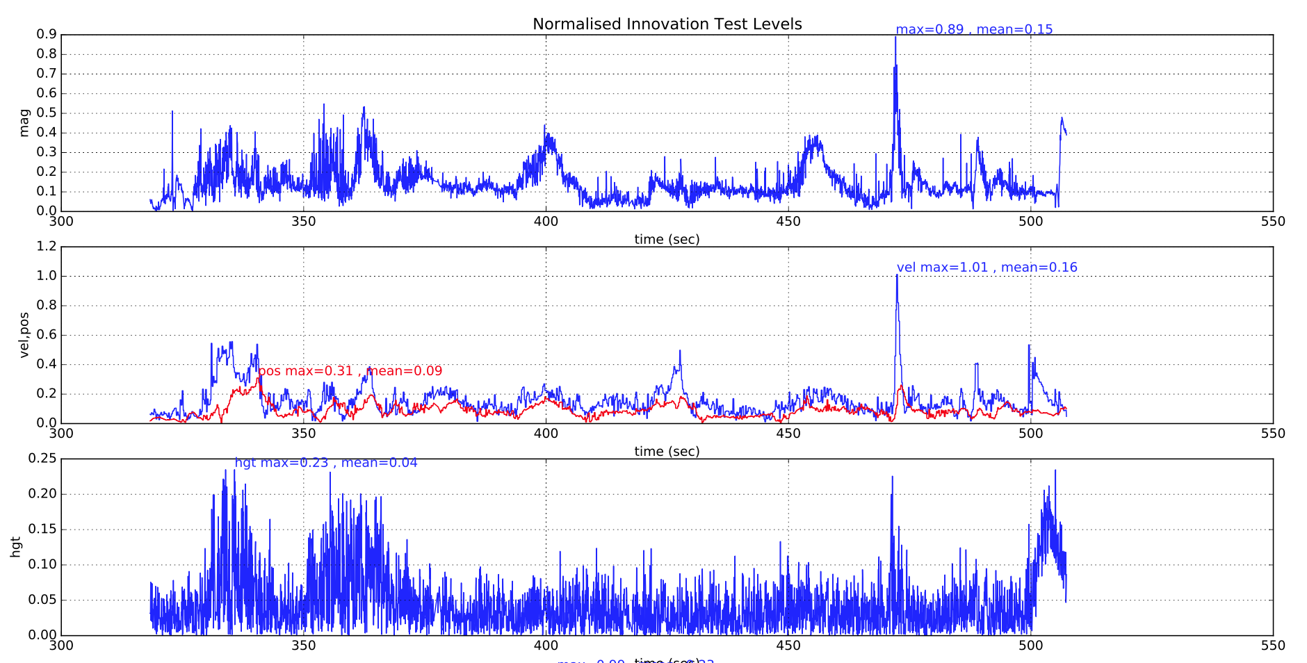
During normal operation, all the test ratios should remain below 0.5 with only occasional spikes above this as shown in the example below from a successful flight:

The following plot shows the EKF vibration metrics for a multirotor with good isolation. The landing shock and the increased vibration during takeoff and landing can be seen. Insifficient data has been gathered with these metrics to provide specific advice on maximum thresholds.

The above vibration metrics are of limited value as the presence of vibration at a frequency close to the IMU sampling frequency (1kHz for most boards) will cause offsets to appear in the data that do not show up in the high frequency vibration metrics. The only way to detect aliasing errors is in their effect on inertial navigation accuracy and the rise in innovation levels.

In addition to generating large position and velocity test ratios of > 1.0, the different error mechanisms affect the other test ratios in different ways:

Determination of Excessive Vibration

High vibration levels normally affect vertical positiion and velocity innovations as well as the horizontal components. Magnetometer test levels are only affected to a small extent.

(insert example plots showing bad vibration here)

Determination of Excessive Gyro Bias

Large gyro bias offsets are normally characterised by a change in the value of delta angle bias greater than 5E-4 during flight (equivalent to ~3 deg/sec) and can also cause a large increase in the magnetometer test ratio if the yaw axis is affected. Height is normally unaffected other than extreme cases. Switch on bias value of up to 5 deg/sec can be tolerated provided the filter is given time time settle before flying . Pre-flight checks performed by the commander should prevent arming if the position is diverging.

(insert example plots showing bad gyro bias here)

Determination of Poor Yaw Accuracy

Bad yaw alignment causes a velocity test ratio that increases rapidly when the vehicle starts moving due inconsistency in the direction of velocity calculatde by the inertial nav and the GPS measurement. Magnetometer innovations are slightly affected. Height is normally unaffected.

(insert example plots showing bad yaw alignment here)

Determination of Poor GPS Accuracy

Poor GPS accuracy is normally accompanied by a rise in the reported velocity error of the receiver in conjunction with a rise in innovations. Transient errors due to multipath, obscuration and interference are more common causes. Here is an example of a temporary loss of GPS accuracy where the multi-rotor started drifting away from its loiter location and had to be corrected using the sticks. The rise in estimator_status.vel_test_ratio) to greater than 1 indicates the GPs velocity was inconsistent with other measurements and has been rejected.

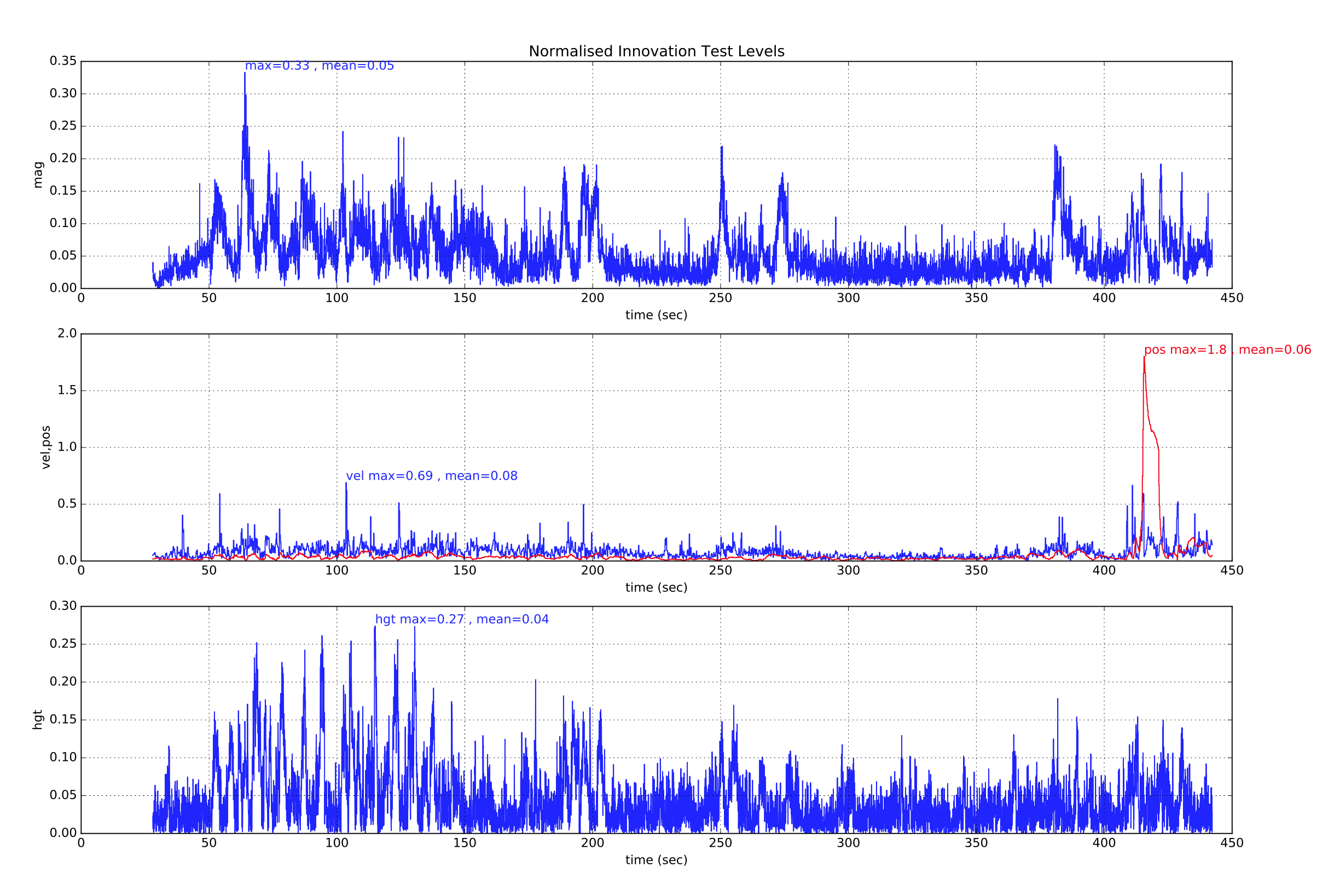
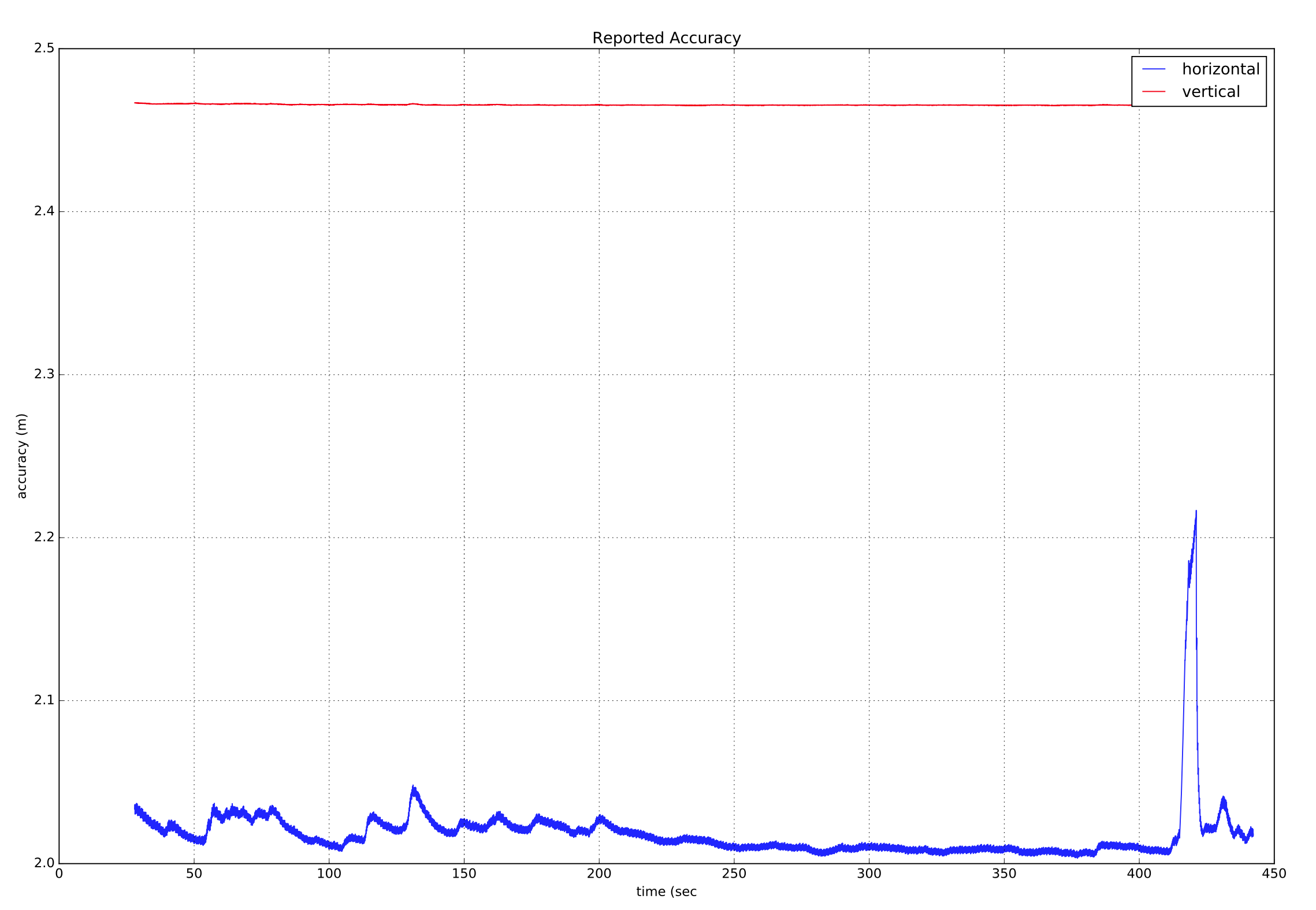
This is accompanied with rise in the GPS receivers reported velocity accuracy which indicates that it was likely a GPS error.

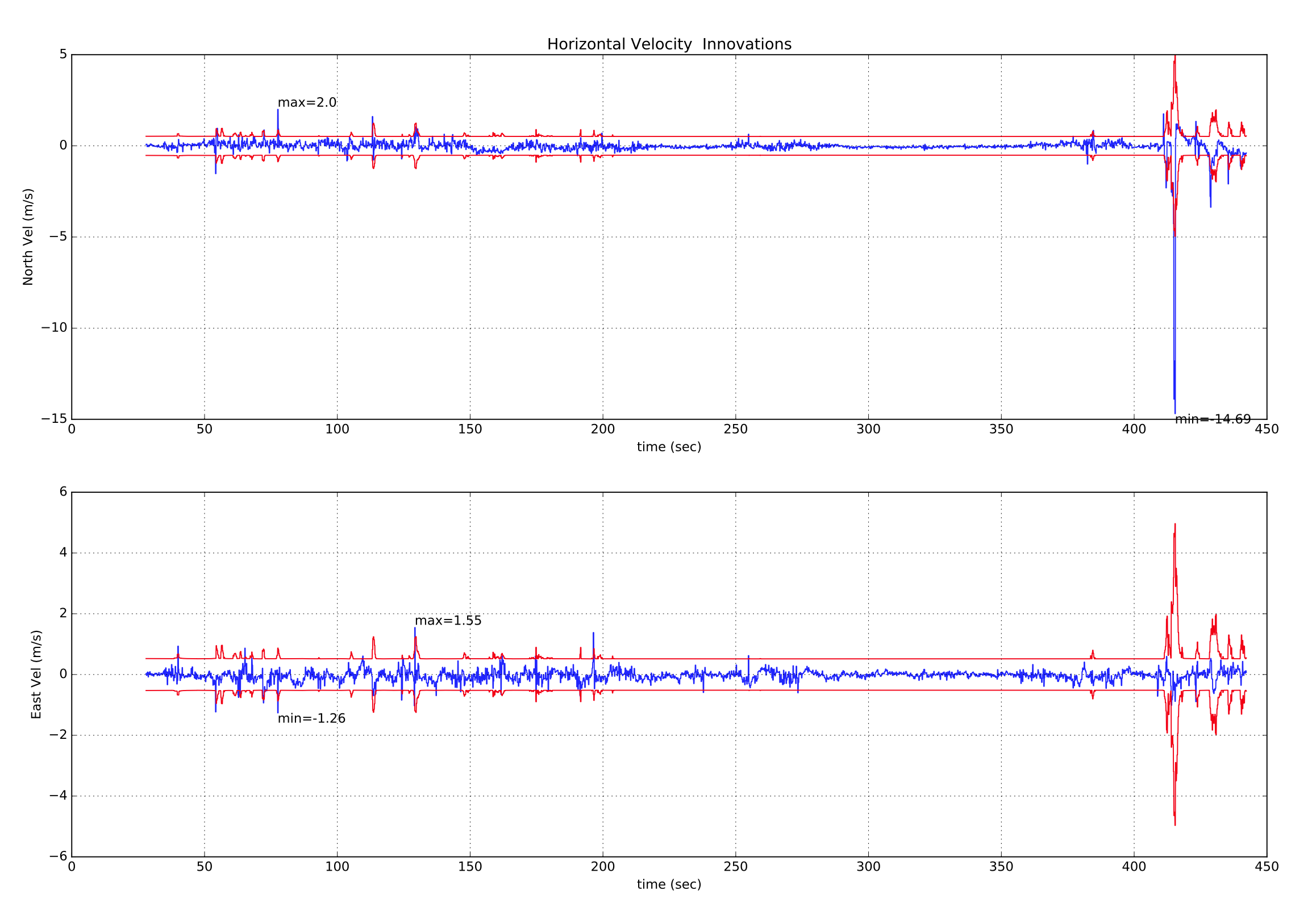
If we also look at the GPS horizontal velocity innovations and innovation variances, we can see the large spike in North velocity innovation that accompanies this GPS 'glitch' event.

Determination of GPS Data Loss

Loss of GPS data will be shown by the velocity and position innvoation test ratios 'flat-lining'. If this occurs, check the oher GPS status data in vehicle_gps_position for further information.

(insert example plosts showing loss of GPS data here)